Pre-post analysis

Introduction

Pre-post analysis is a common statistical approach used to evaluate the effectiveness of an intervention or treatment by comparing measurements taken before and after the intervention. This type of analysis is particularly useful in fields such as medicine, psychology, education, and social sciences, where researchers aim to assess changes in outcomes resulting from specific interventions.

There are two common statistical approaches used for pre-post analysis:

Repeated Measures Analysis of Variance (RM-ANOVA)
Analysis of Covariance (ANCOVA)

RM-ANOVA is used when the same participants are measured multiple times, allowing researchers to account for within-subject variability. ANCOVA, on the other hand, is used to control for potential confounding variables by including them as covariates in the analysis. In this context, the ANCOVA model includes the pre-intervention scores as a covariate. Both models are based on linear regression under the hood, but they differ in how they handle the data structure and the assumptions they make.

Data

We will simulate data for a pre-post study with three groups (for example, two treatment groups and a control group). Each group will have 100 participants, and we will generate pre- and post-intervention scores by drawing from a bivariate normal distribution with specified means, standard deviations, and correlations.

First, we import packages and initialize the random number generator for reproducibility:

library(dplyr)
library(ggplot2)
library(tibble)
library(tidyr)

set.seed(123)

Next, we define the group size:

n = 100

Now, we define the group-specific means for pre- and post-intervention scores:

(means = matrix(
    c(51, 49, 50, 55.5, 53, 52),
    nrow=3,
    dimnames=list(NULL, c("pre", "post"))
))

     pre post
[1,]  51 55.5
[2,]  49 53.0
[3,]  50 52.0

We also define a standard deviation, which we assume to be identical for pre- and post-scores:

s = 10

Finally, we define a correlation between pre- and post-scores:

rho = 0.7

Using these parameters, we create a covariance matrix for the simulated data:

(sigma = matrix(c(s^2, rho * s^2, rho * s^2, s^2), nrow=2))

     [,1] [,2]
[1,]  100   70
[2,]   70  100

We then create a helper function to generate multivariate normal data:

rmvnorm = function(n, mu, sigma) {
    z = matrix(rnorm(n * length(mu)), nrow=n)
    z %*% chol(sigma) + matrix(mu, nrow=n, ncol=length(mu), byrow=TRUE)
}

Using this function, we generate the simulated data for all three groups:

m = do.call(rbind, lapply(1:nrow(means), function(i) rmvnorm(n, means[i, ], sigma)))

df = tibble(
    id=as.character(1:(3*n)),
    group=factor(rep(c("A", "B", "C"), each=n)),
    pre=m[, 1],
    post=m[, 2]
) |>
    pivot_longer(cols=c("pre", "post"), names_to="time", values_to="score")

df[["time"]] = factor(df[["time"]], levels=c("pre", "post"))

Here’s a scatter plot showing the three groups pre- and post-intervention:

means_data = df |>
    group_by(group, time) |>
    summarize(score=mean(score), .groups="drop")

ggplot(data=df, mapping=aes(x=group, y=score, color=time, fill=time)) +
    geom_point(
        position=position_dodge(width=0.5),
        shape=19,
        size=2,
        alpha=0.5
    ) +
    geom_point(
        data=means_data,
        position=position_dodge(width=0.5),
        shape=23,
        size=3,
        color="black"
    ) +
    geom_text(
        data=means_data,
        mapping=aes(label=round(score, 1)),
        position=position_dodge(width=0.5),
        hjust=-0.4,
        size=3,
        color="black"
    ) +
    labs(x="Group", y="Score", color="Time", fill="Time") +
    theme_minimal()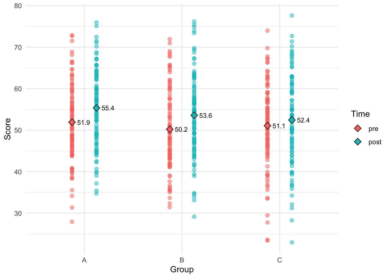

RM-ANOVA

We now analyze the data using an RM-ANOVA model with a within-subject factor time (pre vs. post) and a between-subject factor group (A, B, C):

model1 = aov(score ~ group * time + Error(id/time), data=df)
summary(model1)


Error: id
           Df Sum Sq Mean Sq F value Pr(>F)
group       2    440   220.1    1.38  0.253
Residuals 297  47388   159.6               

Error: id:time
            Df Sum Sq Mean Sq F value   Pr(>F)    
time         1   1126  1126.4  40.316 8.08e-10 ***
group:time   2    139    69.4   2.485    0.085 .  
Residuals  297   8298    27.9                     
---
Signif. codes:  0 '***' 0.001 '**' 0.01 '*' 0.05 '.' 0.1 ' ' 1

We are particularly interested in the group × time interaction, which indicates whether the change from pre to post differs across groups.

ANCOVA

Another common approach for analyzing pre-post data is ANCOVA, where the post-intervention score is modeled as a function of the group and the pre-intervention score as a covariate. This approach adjusts for any baseline differences in pre-scores across groups. Note that we need to expand the time column into separate pre and post columns for this analysis:

df = pivot_wider(df, names_from=time, values_from=score)
model2 = lm(post ~ group + pre, data=df)
anova(model2)

Analysis of Variance Table

Response: post
           Df  Sum Sq Mean Sq  F value  Pr(>F)    
group       2   434.8   217.4   4.4076 0.01299 *  
pre         1 14215.6 14215.6 288.2365 < 2e-16 ***
Residuals 296 14598.5    49.3                     
---
Signif. codes:  0 '***' 0.001 '**' 0.01 '*' 0.05 '.' 0.1 ' ' 1

In this model, we are interested in the effect of group on the post-intervention score.

Furthermore, the additive model assumes equal regression slopes (no group × pre interaction), so we need to check this assumption:

anova(lm(post ~ group * pre, data=df))

Analysis of Variance Table

Response: post
           Df  Sum Sq Mean Sq  F value  Pr(>F)    
group       2   434.8   217.4   4.4363 0.01264 *  
pre         1 14215.6 14215.6 290.1126 < 2e-16 ***
group:pre   2   192.4    96.2   1.9634 0.14222    
Residuals 294 14406.1    49.0                     
---
Signif. codes:  0 '***' 0.001 '**' 0.01 '*' 0.05 '.' 0.1 ' ' 1